Moon lander project: PID-based vs TGO-based guidance
This article is part of a serie: Aerospace simulator
- Moon lander project: thrust vectoring with a PID controller
- Moon lander project: PID-based vs TGO-based guidance
- Moon lander project: preliminary study of the guidance software
As part of my Moon lander guidance software, I am making several small prototypes for each subsystems, in order to test ideas, learn and choose the best option. While I progress on the overall project, I have already learned a lot of things and wanted to share some of them.
In this article, I will talk about how to control the altitude and vertical velocity of a spacecraft in order to guide it to a soft landing. My first (naive) attempt was to use a PID controller. I already have some experience with this kind of controllers and wanted to see if it could work, before researching the canonical solution in the literature and trying more complex options.
Spoiler alert: PID controllers do not work very well, but better than I expected. In this article, I will first demonstrate why a PID is not optimal. Then, I will present the alternative, a TGO-based guidance, which was used during the Apollo program, and is still used today.
Naive approach: PID
Introduction
PID controllers
This short section is not going to be a comprehensive course on PID controllers, but rather a crash course to make sure we are on the same page. If you are looking for a complete explanation, refer to wikipedia or use your favorite search engine.
PID controllers are a kind of control loop mechanism which uses feedback control: it works by computing an error by subtracting a goal value (setpoint) and the current value (measured). This error is used to apply a correction on the system under control. The correction is a weighted sum of three terms: Proportional, Integral and Derivative:
- Term P is proportional to the error. Nothing fancy: small errors give small corrections and big errors give big corrections.
- Term I accounts for past errors. Its goal is to correct the residual error due to a constant force. For instance, when controlling a sailboat with a sideway wind, an I term is needed to avoid missing the targeted position.
- Term D attempts to predict the controller response. It is used to dampen the response of the P and I terms to avoid overshoots.
PID-based guidance
In order to land softly, one need to control both altitude and vertical velocity. These two components must reach zero at the same time. If not, there is a high probability that bad things will happen:
- If the altitude reaches zero while the vertical velocity does not, the spacecraft is obviously crashing.
- If the vertical velocity reaches zero while the altitude does not, it is likely that the spacecraft is wasting fuel and will crash in a near future when it runs out of it.
In order to design a PID-based guidance algorithm, one can design the optimal landing trajectory and then use a controller to follow this predesigned trajectory. This optimal trajectory can be designed by performing an ascent simulation, and running it backwards.
That is exactly what we are going to do.
Descent profile
To generate the descent profile, I refined my algorithm many times. The latest version is quite close to an optimal TGO-based solution, which will allow us to compare similar trajectories.
As said before, the descent profile is actually an ascent trajectory running backward. This ascent trajectory was designed with a TGO controller. I do not want to get too much into the details now, as it will be the next section’s subject. There is only one constraint which I want to highlight: the engine thrust is throttled from 30% to 95% in the first few seconds, to ensure a soft landing (30% is close to the thrust ratio needed to exactly counteract the gravity).
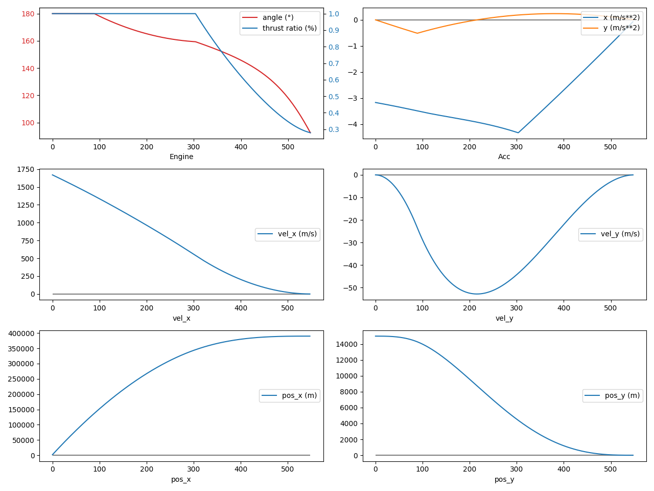
The resulting ascent trajectory is showed below. The first line shows the engine thrust and angle, as well as the net acceleration (including gravity and centrifugal forces). The second line shows the velocity and the thirst line shows the position.
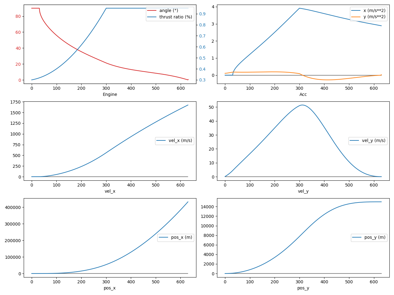
A few things can be observed.
As mentioned, the engine thrust is throttled from 30% to 95% in the first few seconds of the flight, to allow a soft landing. The maximum thrust is 95% to allow the lander to cope with dispersions by regulating the thrust up to 100% if needed. The angle starts at 90° (vertical) and pitches down slowly during the flight to reach 0° (horizontal) once the objective vertical altitude is reached. The resulting acceleration shows that the bulk of the work is done in the x axis, to reach the required orbital velocity of ~1700 m/s. Remember that this is a backward running simulation: the fuel is increasing, not decreasing. That is why the acceleration on the x axis is slowly decreasing between 300 and 600 sec: the spacecraft is getting heavier.
The second line of the plots shows that the x velocity is increasing during the whole flight, as expected from the corresponding acceleration curve. The y velocity starts (takeoff) and finishes (stabilization at a constant altitude) at 0 m/s.
Finally, the x position does not matter much ; and the y position reaches 15 km, which is the standard altitude used by Apollo for a low Lunar orbit.
PID-based guidance demo
With a trajectory designed offline, I can now show the code used to implement the PID controller which will follow this trajectory.
Code
The code is actually relatively simple. It is shown below, heavily commented.
|
|
Tuning
After the code is written, one need to tune the PID weights (Kp, Ki, Kd). The wikipedia page on PID controllers has an (understandably) extensive section on tuning. After spending myself many hours playing with PID weights, I came to the conclusion that the method which has the best quality / time spent ratio is to just use the Ziegler–Nichols method. If your hobby is PID tuning, feel free to spend years doing a thesis. I, myself, like to spend my evenings doing other things, so I’ll just use the work of other smart people.
The first step in PID tuning is to obtain an oscillating response. Once the control loop has stable and consistent oscillations, one can compute the oscillation period, Tu. Different K give different oscillation periods. After trying several K, the following results were obtained:
| Ku | Tu |
|---|---|
| 0.001 | 199 |
| 0.01 | 63 |
| 0.1 | 20 |
| 1 | 6 |
| 10 | 2 |
I choose Ku=0.1 / Tu=20 as a compromise between a (relatively) fast response and an accurate control (no oscillations).
With this ultimate gain Ku=0.01, the Ziegler–Nichols method gives us the final weights for the PID:
- Kp = 0.6*Ku = 0.060
- Ki = 1.2*Ku/Tu = 0.006
- Kd = 0.075KuTu = 0.150
Demo
With these weights, the landing attempt result is shown below. Have a look at the curves, and let’s meet again just after to analyze them together.
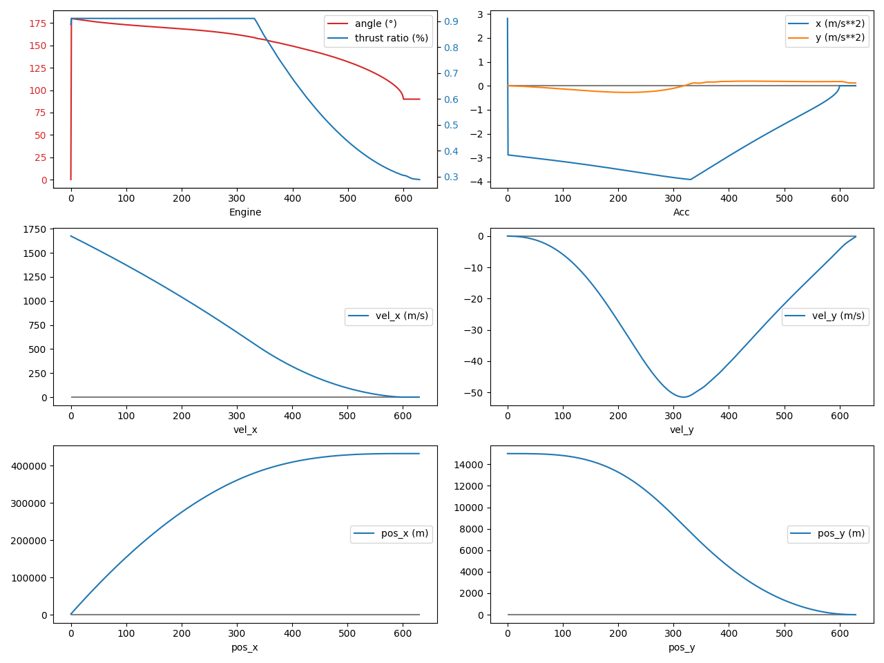
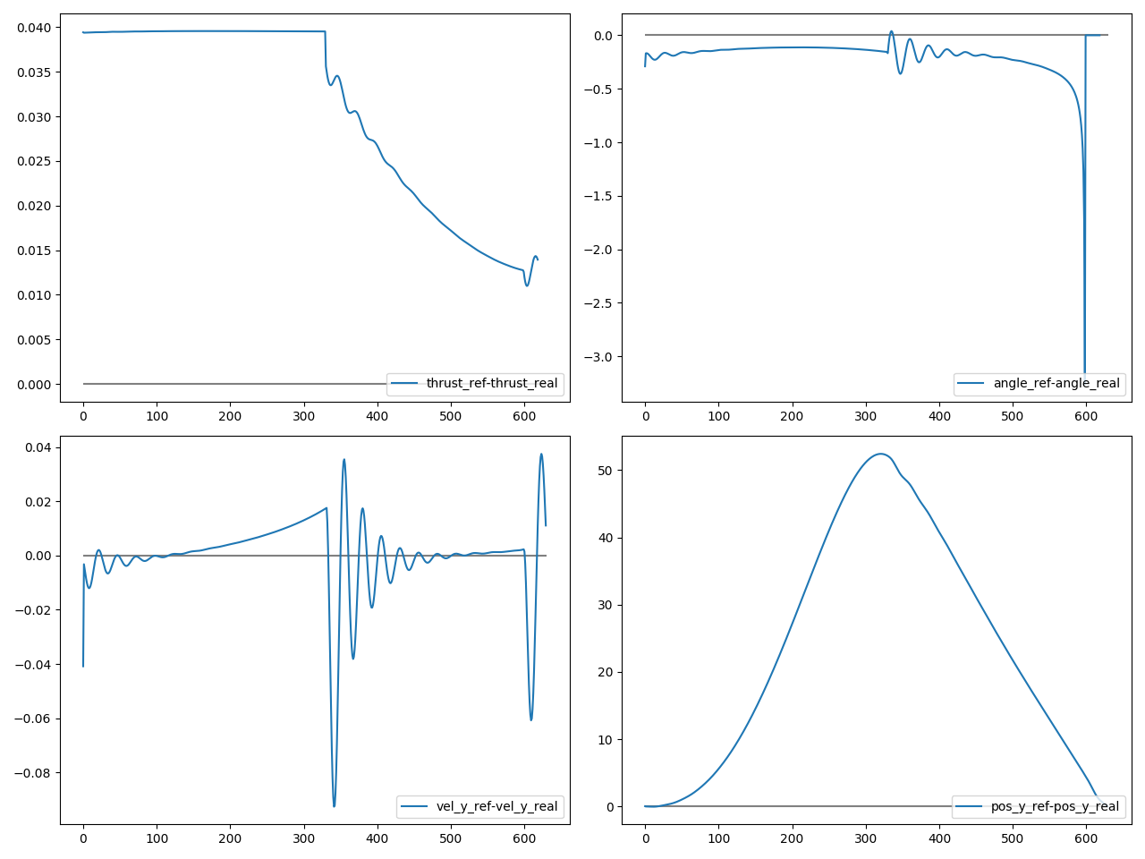
The first graph shows the same data as the previous one, and there is not so much to say about it. Therefore, I will just jump to the second graph, which shows the difference between the reference trajectory and the achieved trajectory.
The first line shows the thrust and angle difference. The achieved thrust is really close to the reference thrust, with a difference of less than 0.1%. The achieved angle is also very close to the reference angle, most of the time under 0.5°. The short spike at 3° could be smoothed out with an angular rate limiter. The achieve thrust and angle following closely the reference ones shows that the PID controller is quite accurate at following the reference trajectory.
Indeed, when looking at the error for the y velocity, it can be seen that it is very close to zero. The y position, is less clear. On one hand, coming from an altitude of 15 km, 50 m of error is quite small. On the other hand, a 50 m error when touching down can be fatal to the mission. The good news is that this error is transient and quickly reaches zero when approaching touchdown. In any case, it does not invite to blindly trusting this landing guidance method.
Note that I am ignoring the x axis here. Although it is important for a good scientific return of the mission (land near what we were supposed to study), it is not critical for a successful landing (avoid killing the astronauts).
Lessons learned
By spending a lot of time fine tuning the PID controller, one can achieve a pretty good response, on the surface. In reality, this method is unreliable and doomed to fail at some point.
As it is implemented in my example, the controller tries to control the position. But it is a lagging indicator of the acceleration, because of the intermediate step which is the velocity. Controlling the velocity instead of the position would be much more simple and effective, but dispersions could add up and the altitude error could reach a very large value at the end, leading to a crash.
Maybe a very conservative altitude trajectory could be followed, with several phases and a dedicated PID for each one… But it will only be more complex and less reliable.
There must be a better way! A single unified control for both the velocity and position is needed. Sadly, a double PIDs will not work, as they would fight each other. The controller needs to understand the underlying physics: the position is the velocity integrated.
Furthermore, the propellant consumption (or rather, the current propellant mass) is important: it impacts the weight and therefore the acceleration of the spacecraft. A PID does not take into account this, and a PID tunned for a specific propellant mass might not work if the spacecraft’s mass changes, for instance if the engine efficiency is mis-estimated.
These difficulties lead us to the other method: TGO-based guidance.
Apollo’s approach: TGO-based guidance
As we saw with a PID controller, there is a need to control both the velocity and the position at the same time. A Time-To-Go (TGO) controller reasons from first principles, using the equations of position, velocity and acceleration, and deriving a control law from them.
Introduction
Designing a TGO-based guidance is relatively easy, once you know what to do. Let’s follow together the few steps which are necessary.
The first part needs to be done only once, offline:
- Choose a Time-To-Go (TGO), which corresponds to the remaining duration of the flight. This is the main concept for this method. With a PID controller, the duration of the control is not explicitly specified, and a best effort approach is used. The TGO is crucial and can be somewhat estimated given the DeltaV amount to achieve and the thrust available, but it will be refined with some simulation, to find one which leaves enough control margin.
- Choose an arbitrary acceleration profile.
This is a polynomial function of
twith parameterski, which can be as simple as a constant, or as complicated as a cubic function. For example, for a linear law:acc(t) = k1*t + k2. Higher order functions will allow to specify more constraints (vel(tgo)=0,acc(tgo)=0, etc), which will give a smoother final trajectory. - Lay down the equations and constraints. The velocity is the acceleration profile integrated, and the position is the velocity integrated. Constraints will be the current (t = 0) and final (t = tgo) position and velocity. If enough parameters are available (high order polynomial), the final (t = tgo) acceleration and jerk can also be used.
- Solve for
ki. The acceleration profile contains unknown (ki) parameters, which are to be solved for. - Simplify the acceleration profile by substituting all the known variables by their values.
The acceleration function should now be a simple function of
tand initial position and velocity.
The second part is done at each control cycle:
- The remaining variables of the acceleration profile function are substituted: tgo, initial position and velocity. This gives you the commanded acceleration, which can now be used to control the spacecraft.
- The commanded acceleration is adjusted with the gravity and centrifugal force (only for the y axis, obviously).
- The engine is gimbaled and its thrust adapted to fulfill the commanded acceleration.
Control law equations
Let’s take an arbitrary acceleration function as an example and derive together the final flight profile.
Apollo used a quadratic acceleration law for the x axis (acc(t) = k1*t**2 + k2*t + k3) and a linear acceleration law for the y axis (acc(t) = k1*t + k2).
Each polynomial order has different advantages and drawbacks, which I will discuss a bit later.
In this example, I will use a quadratic acceleration law.
The code is a bit long and complex, so I prefer not to show it here, but you can find it here. It uses the SymPy Python library, which I have presented in another article.
In the end, I obtain the following acceleration control law: acc(t) = acc(tf) - 6/tgo*(vel(tf)+vel(t0)) - 12/tgo**2*(pos(tf)-pos(t0)).
Checking Apollo’s control law, we see it is exactly the same, which demonstrates that the SymPy code derives the correct equation!
The following graph shows various control functions. The previously-shown quadratic control function is shown in green.
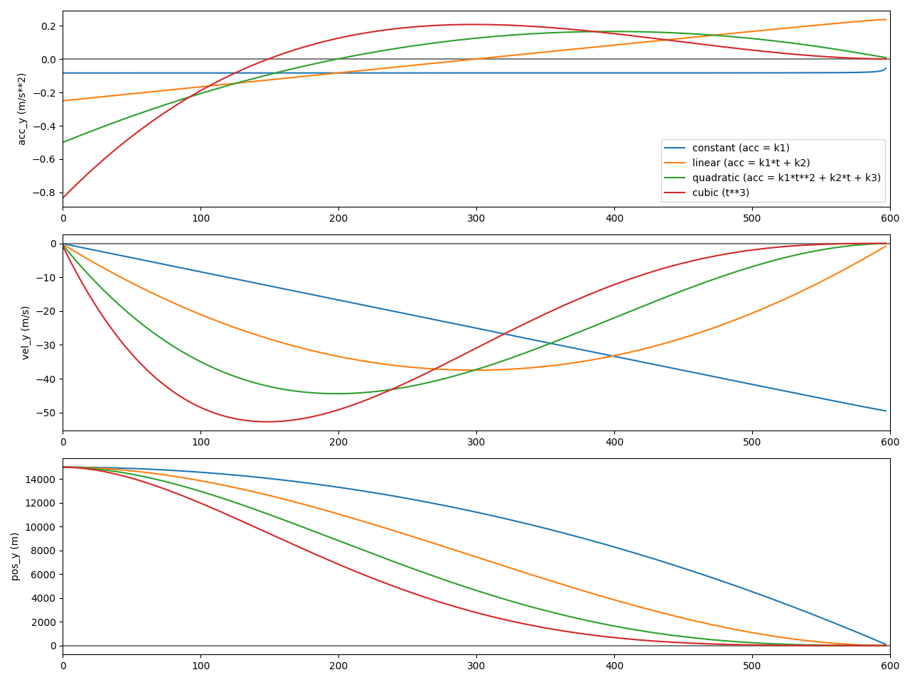
This graph shows that the constant law (blue) lands the spacecraft with a non zero velocity. In other words, the spacecraft crashed.
With a higher order control law, the linear control law (orange) lands the spacecraft with a velocity of zero, but a non zero acceleration. Although the landing is successful, it is not very smooth. A dispersion of the performances could lead the spacecraft to land with a non-zero velocity, meaning crashing. An extensive verification could be done to ensure that enough margin is available, or, alternatively, a higher order control law could be used.
The quadratic control law (green) shows that the acceleration reaches zero at the end, leaving a large margin in the control.
Finally, a cubic control law is a also shown (red). This control law have a landing which is too smooth: it spends too much time very close to the ground, meaning that it wastes fuel and risks hitting a mountain or other land features. A tradeoff must be made between a fast, fuel efficient, but dangerous landing ; and a safe but slow and fuel inefficient landing.
TGO-based guidance demo
To demonstrate a TGO guidance, I implemented an example with the quadratic law presented in the previous subsection, for both the x and y axis.
Constraints
The constraints at tf are the following:
- acceleration x and y: 0
- velocity x and y: 0
- position x: 390 000 (manually tuned for optimal trajectory)
- position y: 0
Nice tricks
The full GNC code has some nice features / optimizations. Here are some of them explained:
- Using the gravity to save fuel: when the guidance orders a negative y acceleration, control orders an horizontal full thrust. This will reduce the x velocity, decreasing the centrifugal force. Of course, this works only with enough margins: time margin, to fall ; and then thrust margin, to reduce the vertical velocity once the guidance has converged.
|
|
- Requested thrust is higher that available thrust: fulfill y, best effort x: in case the requested thrust is bigger than available, the y command is fulfilled, while the x is “best effort”. The goal is to ensure the most critical part is fulfilled (y), because a successful landing far from the objective is better than a crash.
|
|
- Best case: both x and y can be fulfilled:
|
|
TGO determination
The determination of the TGO is critical. In practice, a extensive Monte Carlo campaign is run to find the configuration which gives the best trajectory, but an initial TGO can be estimated with a simple algorithm. This estimated TGO can be used as an initial guess.
The main idea to estimate this TGO is to compute how much DeltaV needs to be achieved.
This is mainly the current spacecraft velocity minus the goal velocity: craft.vel_x - final_vel_x_goal.
With the spacecraft mass, engine thrust, ISP and mass flow, and the Tsiolkovsky rocket equation, I can compute the amount of time needed to achieved this DeltaV.
I also take care of the y axis, and gravity/centrifugal force.
Finally, I multiply by a factor (usually something around 1.10-1.20) to take into account that the engine will not be running at 100% all the time.
Results
Running the simulation with a TGO guidance gives the following result. As usual, give a peek, and let’s meet again after to discuss the curves.
Looking at the first two subgraphs, three phases can be distinguished:
- A first phase until 90 sec: the gravity is used to achieve the commanded vertical velocity. The control function orders a full horizontal thrust to reduce the centrifugal force, and therefore increase the downward force imparted by the Moon. This saves fuel, instead of aiming downward to actively fulfill this negative vertical acceleration.
- A second phase from 90 to 300 sec: full thrust, but with active control of the angle. Only the vertical (y) part of the command is fulfilled, because it is critical to not crash. The horizontal (x) axis is only “best effort”, until the commanded thrust ratio goes below 1. In reality, I am not an expert and maybe this is a mistake: after some quick testing, trying our best on both axis at the same time seems to work too, although I am not sure what are the impacts in terms of performance and margin.
- A third phase from 300 sec until landing: full control is achieved, fulfilling the command of both axis.
The result at the time of landing (tf = 547 sec) is as follow:
- The position error (x axis) is 0 m.
- The velocity error is 0.061 (x) and -0.008 m/s (y). This is very close to 0, and a final phase with a vertical descent during ~30 seconds would most probably reduce this to exactly 0.
- The final thrust ratio is 0.27 and angle is 92.6 degrees. The non-90 degrees angle is due to the x component being to exactly perfect.
Overall, the precision is not perfect, but looks good to me. My goal is to land a spacecraft in KSP, and this should be more than enough.
Margins
Once the algorithm works for a specific set of parameters, an analysis must be performed to assess the stability and the margins: will it still works with the inevitable dispersions of the various sensors and actuators? Usually, the Monte Carlo method is used: many simulation are run with different sets of parameters.
This article is already too long, so I will not delve too much into this topic, but I have done a quick Monte Carlo analysis to determine the influence of the TGO. The constraint I have considered is the remaining amount of fuel at the time of landing.
Here is the (rounded) results:
| TGO (sec) | Fuel left (kg) |
|---|---|
| 520 | 7750 |
| 550 | 7700 |
| 580 | 7600 |
| 610 | 7400 |
One can see that the larger the TGO is, the smaller the remaining fuel is, which makes total sense. When the TGO is too small, the thrust ratio remains above 1.0 and the controller angle can jump. The best compromise for the TGO seems to be around 550 seconds.
Conclusion
This article is already very long, so I will stop here.
PID vs TGO
With this article, I have found out that a PID controller works better than expected. The downside is that it needs a well-designed trajectory, and good performances require a lot of manual tuning.
Apollo’s method, TGO guidance, works really well (of course, they landed humans on the Moon after all). Once the method is understood, TGO is very simple to implement.
TGO guidance can be seen a bit like a simple P controller (without I nor D), but instead of following the objective trajectory and oscillating around it, it just adapts and recalculate a new trajectory satisfying the constraints. In other words, TGO guidance will not saturate like a PID, and will be better at recovering trajectory dispersions.
The main risk of TGO is to go out of the flight envelope, but with an extensive Monte Carlo analysis, it can be proved that there is enough margin.
Future work
The physic simulator used, which I implemented, is very crude and ignores a lot about:
- Engine performance
- Propellant sloshing
- Sensors/astronaut/payload constraints (for ex: visibility) and precision (for ex: altitude bias and noise)
The next steps will be to, first perform an extensive margin assessment with a Monte Carlo analysis, and then, implement this TGO guidance and the full simulator in Rust and connect it to KSP.
References
You can find the list of all the Python source files here and an archive here. I wrote all the code myself. The lander used in all the examples is based on Apollo, you can find the detailed spec in the code in utils/space.py and utils/sim.py.
I read many papers on guidance and Apollo. Here are a few of them:
- NASA technical memorandum and note:
- Apollo lunar descent and ascent trajectories (by Floyd V. Bennett, March 1970, original link): Apollo’s guidance law is shown on page 7.
- Apollo experience report - mission planning for lunar module descent and ascent (by Floyd V. Bennett, June 1972, original link): contains more details than the previous paper, and Apollo’s guidance law is also shown on page 12.
- Apollo lunar-descent guidance (by Allan R. Klumpp, June 1971, original link): contains a breakdown of the various Apollo landing phases.
- More recent work on descent guidance:
- An optimal guidance law for planetary landing (by Christopher N. D’Souza, 1997, original link)
- Powered descent guidance methods for the Moon and Mars (by Ronald R. Sostaric and Jeremy R. Rea, 2005, original link): contains some interesting information about guidance law, time-to-go and optimal guidance.
- Finally, a very well explained Master of Science thesis:
- Comparison of Guidance Methods for Autonomous Planetary Lander (by Wyatt Harris, April 2011, original link): the chapter 3, Guidance Methods, is especially interesting to understand time-to-go and guidance laws.