Symbolic maths in Python: Attacking a castle with SymPy

• 2020-11-21
• Dev  

While working on my Moon lander guidance software, I am making several small prototypes to test ideas. One of them involves testing several control laws (of the acceleration), which implies quite a lot of manual calculations (to integrate to obtain the velocity and position).

Doing these calculations by hand is tedious and error prone, and I thought about using a symbolic math program. Usually, a programming language can not manipulate variables without predefined values, but I found a Python library which can: SymPy.

This article will serve as a small demonstration of its capabilities, and to do so, we will jump a few centuries before rocketry was invented: let’s attack a castle!

SymPy basics

The main point of SymPy is that it understands maths. For example, with the standard Python library, computing math.sqrt(8) will gives us 2.82842712475. For engineers, this is not really false, but for mathematicians, it is not really true either. If you ask SymPy, sympy.sqrt(8) gives 2*sqrt(2), which is mathematically exact.

Symbols

Before doing anything with SymPy, you need to declare the symbols you will use in your expressions.

Let’s declare a symbol x, and compute the arbitrary expression cos(x)**2 + sin(x)**2.

 1
 2
 3
 4
 5
 6
 7
 8
 9
10

# Source: example_1_1_symbols()

import sympy as sp

x = sp.symbols('x')

expr = sp.cos(x)**2 + sp.sin(x)**2

print(expr)                             # Shows: sin(x)**2 + cos(x)**2
print(sp.simplify(expr))                # Shows: 1

The first print shows sin(x)**2 + cos(x)**2, showing that SymPy has understood the expression. The second print shows 1, as expected (if you remember your math lessons).

Symbols are very powerful, and they allow SymPy to do smart things, such as integrating an acceleration to obtain the velocity. With plain Python; you would not be able to do that.

Mathematical operations

SymPy’s documentation puts it well, so I’m just going to quote it:

The real power of a symbolic computation system such as SymPy is the ability to do all sorts of computations symbolically. SymPy can simplify expressions, compute derivatives, integrals, and limits, solve equations, work with matrices, and much, much more, and do it all symbolically

SymPy’s documentation - The Power of Symbolic Computation

Compute integrals? Let’s try this!

 1
 2
 3
 4
 5
 6
 7
 8
 9
10
11
12
13
14
15

# Source: example_1_2a_math_expr_a()

import sympy as sp

x, a, b = sp.symbols('x a b')

# definite integral of x**2 between 0 and 1
expr = x**2
integrated = sp.integrate(expr, (x, 0, 1))
print(integrated)                       # Shows: 1/3

# indefinite integral of ax+b
expr = a*x + b
integrated = sp.integrate(expr, x)
print(integrated)                       # Shows: a*x**2/2 + b*x

Note that the constant is not automatically added to the integrated expression, because it is not as easy as it looks, for example for expressions with multiple variables. You will need to do it manually, with the knowledge of the context around the problem you are solving, which SymPy can not do. Feel free to look at the Github issue(s) for more info.

Symbolic computations allows you to do all sorts of manipulation symbolically, and plug values in at the last time. Substituting values is done with the subs() function.

What is the value of the integral of f(x) = x**2 for x=1?

 1
 2
 3
 4
 5
 6
 7
 8
 9
10
11
12

# Source: example_1_2b_math_expr_b()

import sympy as sp

x = sp.symbols('x')

expr = x**2
integrated = sp.integrate(expr, x)
print(integrated)                       # Shows: x**3/3

value_at_1 = integrated.subs(x, 1)
print(value_at_1)                       # Shows: 1/3

Predicting a cannonball shot

Now that you understand the basics of SymPy, let’s dive deep by modeling the trajectory of a cannonball. We’re going to start with the acceleration, and integrate it to obtain the velocity and position. Later, we will plug values in for the shooting angle, initial velocity and other constants and compute the trajectory.

Variables and equations

First, we define a few symbols for our time variable (t), constant (g), and parameters (v0, angle). When defining the symbols, we pass some additional information to help SymPy when manipulating the expressions. When solving equations later, it will prevent SymPy from giving us nonsensical solutions (for example, negative time).

We then define the equations, starting with the acceleration. There is only g (if the castle you are attacking is on a windy hill, feel free to add it). Additionally, the initial velocity in the x and y axis depends on the angle, and the initial position is zero.

Thanks to SymPy and its integration feature, the final equations are calculated automatically.

 1
 2
 3
 4
 5
 6
 7
 8
 9
10
11
12
13
14
15
16
17
18
19
20
21
22
23
24
25

# Source: example_2a_cannonball_shot_eq()

import sympy as sp

t = sp.symbols('t', real=True, positive=True)
g = sp.symbols('g', real=True, positive=True)
v0, angle = sp.symbols('v0 angle', real=True, positive=True)

G = 9.81

acc_x = 0
acc_y = -g

vel_x = sp.integrate(acc_x, t) + v0*sp.cos(angle)
vel_y = sp.integrate(acc_y, t) + v0*sp.sin(angle)

pos_x = sp.integrate(vel_x, t)
pos_y = sp.integrate(vel_y, t)

print('acc_x =', acc_x)                 # Shows: acc_x = 0
print('acc_y =', acc_y)                 # Shows: acc_y = -g
print('vel_x =', vel_x)                 # Shows: vel_x = v0*cos(angle)
print('vel_y =', vel_y)                 # Shows: vel_y = -g*t + v0*sin(angle)
print('pos_x =', pos_x)                 # Shows: pos_x = t*v0*cos(angle)
print('pos_y =', pos_y)                 # Shows: pos_y = -g*t**2/2 + t*v0*sin(angle)

Calculating the trajectory

Second, we calculate, for each t, the position.

The only thing to pay attention to, is to not mix up a SymPy variable and its value. In my examples, the SymPy variables are lowercase (for ex. g), while the values are uppercase (G).

float() is used to force SymPy to compute an actual value. With this simple example, it is probably not needed, but in more complex cases, it can be useful to ensure that SymPy actually computes a value. If it can not, and the expressions still has variables, it will fail loudly (raise an exception), allowing you to debug and fix the code.

 1
 2
 3
 4
 5
 6
 7
 8
 9
10
11
12
13
14
15
16
17
18
19
20
21
22
23
24
25
26
27
28

# Source: example_2b_calc_traj()

V0 = 50
ANGLE = deg2rad(42)
TMAX = 200

# Simplify a bit the equation now

pos_x_t = pos_x.subs(v0, V0).subs(angle, ANGLE)
pos_y_t = pos_y.subs(g, G).subs(v0, V0).subs(angle, ANGLE)

print(pos_x_t)                          # Shows: 37.1579645676346*t
print(pos_y_t)                          # Shows: -4.905*t**2 + 33.4557270013732*t

# Compute the trajectory until the cannonball hits the ground, with a 0.1 sec increment

pxs, pys = [], []

for T in np.linspace(0, TMAX, TMAX*10+1):
    px = float(pos_x_t.subs(t, T))
    py = float(pos_y_t.subs(t, T))

    # we have hit the ground? Then break
    if py < 0:
        break

    pxs.append(px)
    pys.append(py)

Results

The previous code is run for several angles (20°, 30°, 40°, 50°), and the trajectory is plotted.

It can be seen that the furthest impact is at around 250 m, for an angle of 40° and 50° (the maximum range of the cannon is probably with an angle of 45°, at around 230 m).

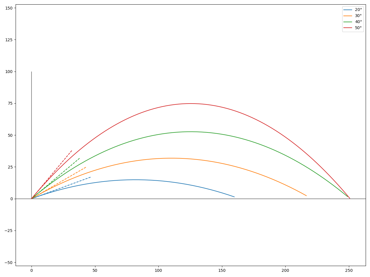
With a handful of lines of code and absolutely no manual calculations, SymPy perfectly answers our problem of modeling a cannonball.

Attacking a castle

Before we attack the fortress, my French-speaking readers will enjoy rewatching this excerpt from a masterpiece of the French’s seventh art.

While we wait for those who clicked the link to come back, let me introduce you with our target. This castle seems a bit crude, but I am sure it is a very cozy place once fully furnished and heated. Let’s attempt to conquer it!

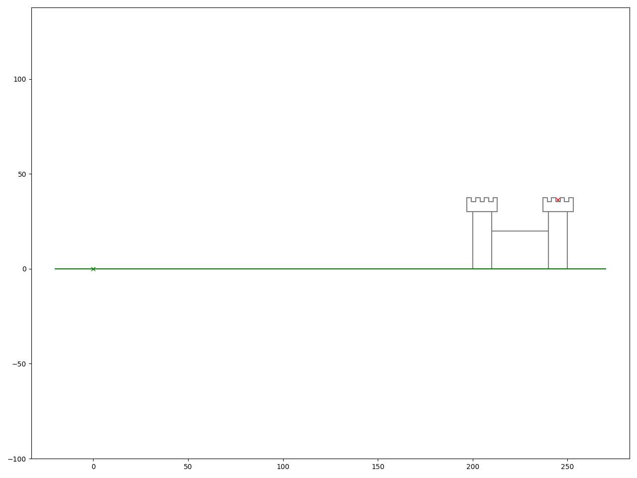
Our soldiers just spotted the king in the second tower! There is not a lot of time to kill him, and we probably have only one attempt before he hides.

At which angle should we shoot the cannonball? We already know the motion equations, and thanks to our engineers and surveyors, we now know the target coordinates: (245, 37), and the initial velocity of the cannonball: 60 m/s (I’m a software engineer, not a fireworks operator, so I’m going to take their word for it).

 1
 2
 3
 4
 5
 6
 7
 8
 9
10
11
12
13
14
15
16
17
18
19
20
21
22
23
24
25
26
27
28
29
30
31
32
33
34

# Source: example_3b_attack_v0_60()

V0 = 60
TARGET_X = 245
TARGET_Y = 36.5

# Let's do so substitutions/simplifications before the heavy calculation
pos_x_t = pos_x.subs(v0, V0)
pos_y_t = pos_y.subs(g, G).subs(v0, V0)

# The meat of the solver is here. The two arrays passed as arguments are:
# 1. Equations to solve ("sp.Eq(pos_x_t, TARGET_X)" means "pos_x_t == TARGET_X")
# 2. Variables to solve for
sols = sp.solve([
    sp.Eq(pos_x_t, TARGET_X),
    sp.Eq(pos_y_t, TARGET_Y),
], [angle, t])

# Let's get all the valid solutions
# When declaring SymPy symbols, we specified that angle and t were positive, so
# all solutions should be valid (no negative times or velocity).
sols_v0_60 = []  # angle_rad, t
for (angle_sol, t_sol) in sols:
    sols_v0_60.append((float(angle_sol), float(t_sol)))

# Print the solutions
print('v0: angle_deg t')
for (ANGLE_RAD, T) in sols_v0_60:
    print('%d: %d %4.1f' % (V0, rad2deg(ANGLE_RAD), T))

# The above code prints:
# v0: angle_deg t
# 60: 31  4.8
# 60: 67 10.6

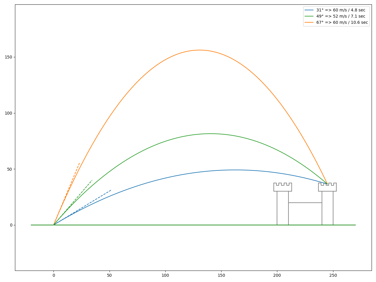
So, for a given initial velocity of 60 m/s, there are two solutions to hit the enemy king: one with an angle of 31° (time of flight 4.8 sec) and one with an angle of 67° (time of flight 10.6 sec).

If we are short on powder, we can compute the parameters for a shoot to save as much as possible. To achieve this, we will solve for the point where the initial velocity is minimal, which is where the derivative of the initial velocity is 0.

 1
 2
 3
 4
 5
 6
 7
 8
 9
10
11
12
13
14
15
16
17
18
19
20
21
22
23
24
25
26
27
28
29

# Source: example_3c_attack_v0_min()

TARGET_X = 245
TARGET_Y = 36.5

pos_y = pos_y.subs(g, G)

# Similar as before, solve for v0
sols = sp.solve([
    sp.Eq(pos_x, TARGET_X),
    sp.Eq(pos_y, TARGET_Y),
], [v0, angle])
assert len(sols) == 1
v0_sol, angle_sol = sols[0]

# Once we have v0, solve for t when its derivative over t is equal to 0
sols = sp.solve([sp.diff(v0_sol, t)], [t])
assert len(sols) == 1
(t_sol, ) = sols[0]

# Finally, reduce all the variables
v0_min = float(v0_sol.subs(t, t_sol))
angle_at_v0min = float(angle_sol.subs(t, t_sol))
t_at_v0min = float(t_sol)

print('v0_min = %.1f' % v0_min)                     # Shows: v0_min = 52.8
print('angle_deg = %.1f' % rad2deg(angle_at_v0min)) # Shows: angle_deg = 49.2
print('t = %.1f' % t_at_v0min)                      # Shows: t = 7.1

On the following graph, you can see the previously mentioned v0 = 60 m/s shots, with our beautiful minimal shot with v0_min = 52.8 m/s.

Conclusion

In this article, I hope to have given you a good overview of SymPy’s features and how to use it.

I used a simple example to demonstrated some of SymPy features: using symbols, substituting values, applying mathematical operations such as integration, and solving equations. Through this basic example, I have highlighted in which cases SymPy can be useful: problems which have many parameters. In particular, an aerospace study (where the spacecraft have many parameters: mass, thrust, etc) can greatly benefit from this tool. Coupled with matplotlib for plotting, SymPy is 🔥!

In the future, I will keep SymPy in my toolbox, and remember to use it when appropriate. In particular, I plan to study various guidance control laws for my Moon lander guidance software (next article incoming). Once I have a good understanding of guidance, I plan to design various spacecraft in KSP and fly them. In this case, SymPy will probably be helpful to dynamically adapt to the different configurations.

I will probably not use SymPy very often, but when needed, it will save me a lot of time and avoid errors. I find it crazy that such a library exists, or is even possible. FOSS = <3.

Note: the source code is available here.