Aerospace simulator /

Moon lander project: thrust vectoring with a PID controller

• 2021-04-18
• Aerospace  
• GNC  

The goal of my Moon lander guidance software series is to learn and gain some experience with an end-to-end aerospace software project, especially on the topic of GNC. I have already written a few articles sharing my findings: for instance, this one about guidance.

Today I want to talk about control. I will use the engine gimbal controller of my Moon lander¹ project to explain how to design, tune and validate a PID controller. I will first explain how the control algorithm is designed as a two-steps process with first a translation and then a rotation controller. I will then detail how I designed the rotation controller, which is responsible for the engine gimbal. Finally, I will show the implementation and explain how the performances were validated.

Translation vs rotation control

The control of the spacecraft is implemented as a two-steps process: first, a translation controller, and then, a rotation controller. This naming is probably not industry standard at all, so let’s explain each one in details.

The translation controller takes as input the guidance acceleration commands x and y, and outputs a thrust and an angle. The idea is to determine the ideal angle the rocket should be pointed at, as well as its thrust, to fulfill the commanded guidance. This assumes that the rocket points magically and instantaneously to the commanded angle: it does not takes into account engine gimbal. This translation control is easy: there are no PID controller, no overshoot, no steady state error. It is only some basic trigonometry. The code, implemented here is just under 30 lines. The controlled thrust is a simple function of the commanded acceleration and the spacecraft’s mass: ctr_thrust = gui_acc * sc_mass. The controlled angle is the output of the arctan function: ctr_angle = atan2(gui_acc.y, gui_acc.x).

With a commanded rocket thrust and rocket angle, the second step of the control can take place. It determines the actual engine gimbal that will bring the rocket to the previously determined rocket angle. This rotational control is a bit more complicated: first of all, we have a commanded rocket angle, and (obviously) a current rocket angle. From these, we can derive an angle error, which we want to correct (bring to zero). We will need a controller, as there are no analytically perfect solution. We also have many other sources of complexity, such as the inertia of the spacecraft, or the engine gimbal limits (angular position and velocity).

This article focuses on this second step of the control. We will see together how to design, implement and tune, and finally validate the controller.

Controller design

Unlike the example used in this article (control), the guidance is time-bounded and needs to take into account both position and velocity, which means it needs something smarter than a PID. In our case, for control, the engine gimbal is not time-bounded (it must follow a moving setpoint the best it can), and there is only one variable to control (the gimbal angle). Therefore, a PID fits very well this problem.

The PID’s input (setpoint) will be the commanded thrust angle. The PID’s process variable (the measured value) will be the current spacecraft angle. This seems to be a standard, easy PID controller: compute the error (process variable minus setpoint), and compute the PID’s output (commanded value).

This output control value is not directly the engine gimbal angle, but merely a spacecraft-related angular control. Indeed, there are a two constraints to keep in mind which require this generalization. First, the engine gimbal has a maximum angular position and angular velocity². This is rather easy to manage and will be handled with saturation of the control output. Second, the mass (and therefore the moment of inertia) of the spacecraft changes. This needs to be taken into account somewhere in the control, to avoid having a PID performing well for only a particular mass and badly for other masses.

Controller implementation and tunning

Now that the controller is designed, let’s implement it in Rust.

After the implementation, we will need to tune it to determine the gains Kp and Kd. The goal will be to find a couple (Kp, Kd) which gives a fast response with minimal overshoot.

Implementation

The PID’s implementation is rather simple, so I will not go too much into the details. Just two details. First, the I term is kept at zero, because in space (no atmosphere) there can not be steady state disturbances on the spacecraft. Second, instead of using the derivative of the error, derr, for Kd , I directly use the spacecraft’s angular velocity sc_ang_vel (which is the derivative of sc_ang_pos). This makes sure that Kd applies only on the spacecraft’s behavior, without the disturbances from the commanded angular position ctr_ang_pos.

The code is in Rust, with type hints to make the units more clear. It also uses the uom crate, to avoid mixing units.

1
2
3
4
5
6
7

    // ang acc PID

    let err: Angle = ctr_ang_pos - sc_ang_pos;
    let derr: AngularVelocity = sc_ang_vel;
    let control: Angle = (kp*err + kd*derr).into();

    let ctr_ang_acc: AngularAcceleration = (control * control_transfer_function).into();

The control_transfer_function is a simple factor to scale the PID’s output into something which makes more sense and can be used to actually control the spacecraft. In my case, it is a factor of 1/sec**2 (in fact, only the unit is important), to convert an Angle into an AngularAcceleration.

The angular acceleration can then be converted into a gimbal angle, taking into account the dynamics of the spacecraft (mass, thrust, etc). The last step is to check the engine physical limits (angular velocity and angle).

 1
 2
 3
 4
 5
 6
 7
 8
 9
10
11
12
13
14
15
16
17
18
19
20
21

    // compute torque for correction
    // Inertia: 1/2*m*r**2 = kg.m**2
    // Torque: N*m = kg*m**2 * rad/sec**2

    let sc_moment_of_inertia = 0.5 * sc_mass * squared!(conf.sc_width/2.0);
    let ctr_torque: Torque = (ctr_ang_acc * sc_moment_of_inertia).into();

    // compute engine gimbal
    // Torque = L*F*sin(gimbal)

    let sin_gimbal: Ratio = ctr_torque/(conf.sc_height/2.0*cur_thrust);

    let mut ctr_eng_gimbal: Angle = sin_gimbal.asin();

    // apply engine gimbal limits (angular velocity and angle)

    // [...]

    ctr_eng_gimbal = saturate(
        ctr_eng_gimbal, -conf.ctr_eng_gimbal_pos_max, conf.ctr_eng_gimbal_pos_max,
    );

Tunning

To find the gains Kp and Kd that give the best performances, I simulate the above PID controller with a standard step response. In my case, the measure of the performance is the settling time tau, which denotes the time it takes for the system to reach and stay within 90-110% of the setpoint. The lower this value is, the better.

The 90-110% value is the amount of overshoot which I consider acceptable. I assume that the exact value does not matter too much: the best (Kp, Kd) couple for 90-110% of the setpoint will be the same for 95-105% or 80-120%. I’m mainly interested in the relation between tau, Kp and Kd. I also assume that a sufficiently small tau will not give any oscillations, hence no (or minimal) overshoot: each oscillation outside 90-110% of the setpoint would increase the value of tau, making it not sufficiently small. In any case, after finding potentially good gain values, I will run some landing simulations, asses how stable the spacecraft is, and adjust them accordingly.

Here are the step responses for two differently tunned PIDs; both with a setpoint of 2 degrees. The first one, in blue, uses some default and low values for Kp and Kd (2 and -0.5, respectively). The second one, in orange, uses optimally tunned values for a tau of 0.5 sec: 12.1 and -3.7. The most interesting subplot is the first one, showing the angular position of the engine gimbal. Vertical bars denote the settling time tau for both controllers.

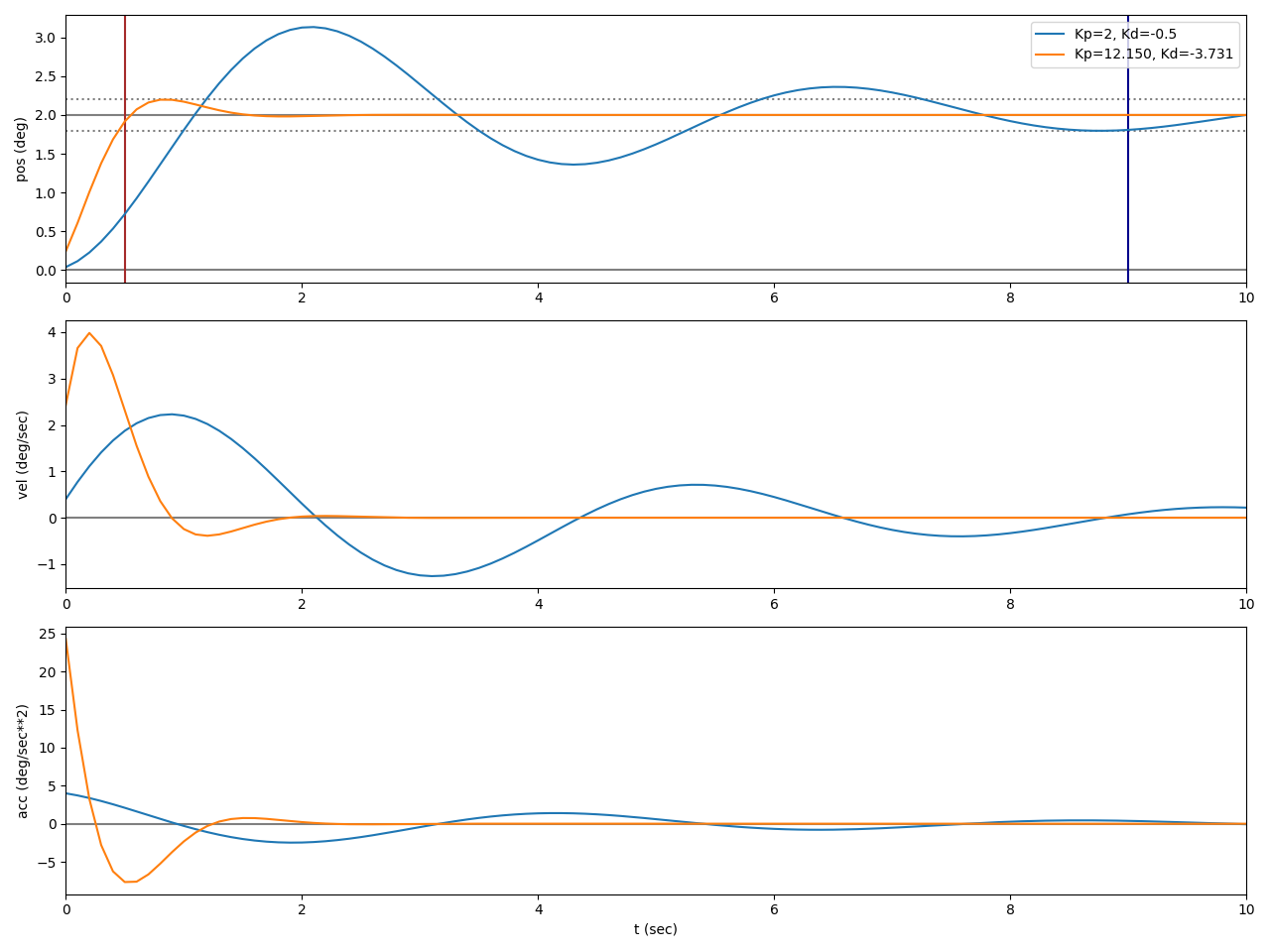
This first PID has a time constant tau of 9.0 seconds. It shows a large overshoot (~50% at 2 sec) and many oscillations before finally settling. The second PID has a time constant of 0.5 second. As I assumed, it settles very quickly and shows almost no oscillations. Clearly, the first one is not optimized, while the second one is.

One thing to keep in mind, which I did not took into account in the step response here, is the maximum angular acceleration that the engine gimbal can achieve: the first controller commands up to ~4 deg/sec², while the second controller commands between 20 and 25. The engine gimbal can achieve a maximum angular acceleration of somewhere between 3 and 9 deg/sec². This depends on the engine thrust and spacecraft mass (and a few other parameters which are constant during the flight, such as the inertia or the maximum gimbal angle). To avoid an unpredictable controller, the controller should be tunned to avoid too strong commands that are outside of the engine’s physical limitations.

To obtain a small tau, the PID needs a large Kp, to have a strong and quick correction. But this comes at the expense of overshoot and oscillations. Kd can be decreased (below zero, hence increase its absolute value) to avoid them. Kd takes into account the angular velocity, and the larger it is, the more it reduces the correction. This makes the PID braking in anticipation when moving too fast toward the setpoint.

In short: a small tau (big Kp) gives a fast correction, with large gimbal commands, and sometimes some overshoot and oscillations (depending on Kd, up to a certain amount). This tunning is good for a short flight, such as a 150 m hop (30 sec). Big tau (small Kp) gives a slow, smooth correction, with small gimbal commands and small to no overshoot. This is suitable for long flights, such as a landing (700 sec).

From Kp and Kd to tau

I’m lazy, and I want to specify only one parameter, not two (Kp and Kd). This one parameter is obviously tau, from which we can estimate the two gains.

Therefore, I need to determine two functions Kp = f(tau) and Kd = g(tau). I will test all (Kp, Kd) couples, find their corresponding tau with a step response, and finally compute a regression of Kp and Kd as a function of tau. I used scipy.optimize.curve_fit to compute the regression, which proved easier than anticipated. The regression uses a power function f(tau) = k_scale * tau**k_exponent to fit the data. A few other regression functions were tested (linear, exponential) but did not fit as well.

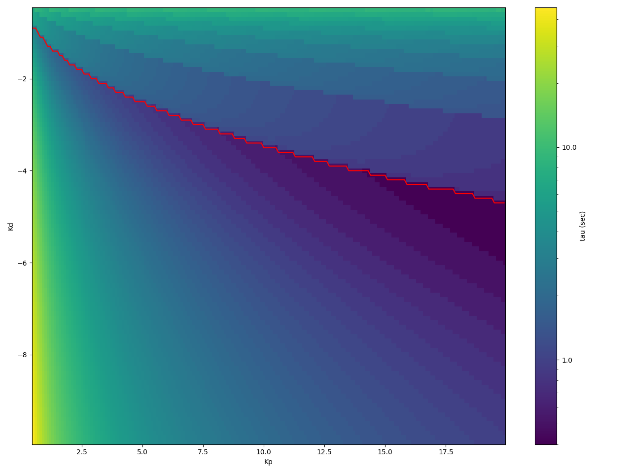
The result is shown below. The first plot shows tau, in function of Kp and Kd. The red line highlights the lowest tau, for a given Kp. The second plot shows Kp and Kd as a function of tau, with the calculated regression.

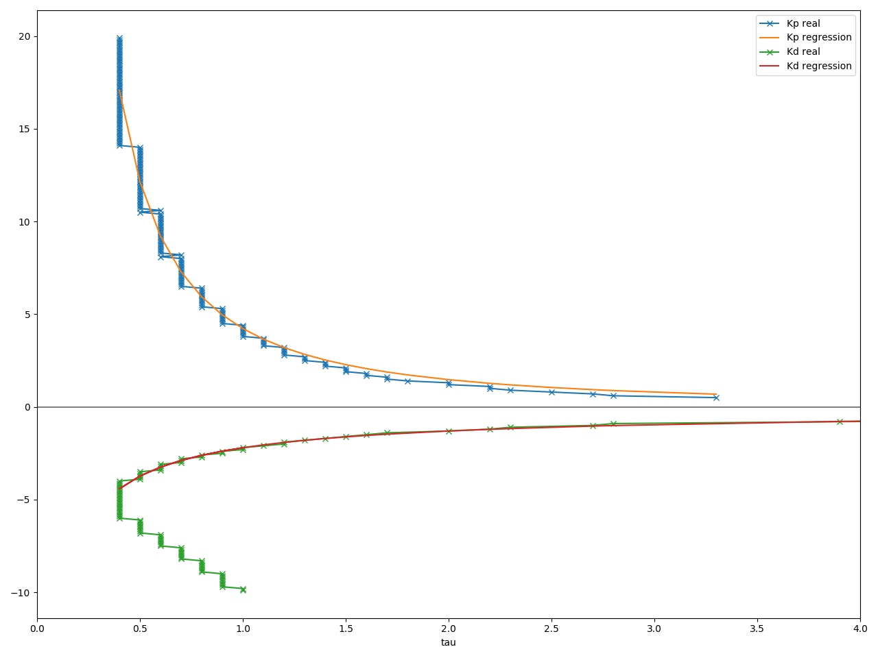
The result of the regression is:

kp_scale = 4.224639
kp_exponent = -1.524106
kd_scale = -2.203941
kd_exponent = -0.759514

For example, for tau=0.5, Kp will be 4.224639*0.5**-1.524106 = 12.150 and Kd will be -2.203941*0.5**-0.759514 = -3.731 (these are the values I used in the step response in the previous section).

Conclusion

This was a fun little subproject. I touched many different things: control theory (PID), Geogebra (for the animated gimbal), Dia (for the block diagram), matplotlib (for the other graphs), programing (Rust, Python), maths (regression), etc. I also learned and practiced some GNC. Even if it is not state of the art, it is still interesting, and good enough for many applications, including my little toy project. All the source files (code and diagrams) can be found in this archive.

I improved my GNC software step by step, learning new things and writing blog articles along the way. First, I assumed that the engine gimbal and the rocket are rigid and point immediately and perfectly the setpoint. Then, I introduced the engine gimbal and the rocket inertia, which created the need for a controller. Later I will add some noise (sensor noise, engine gimbal misalignment, etc) to perfect the simulation.