Free-return trajectory around the moon /

Flying to the moon with Apollo

• 2019-06-05
• Aerospace  

About 50 years ago, humans landed on the Moon for the first time. I initially wanted to write on this subject because I like rockets and space, but this anniversary is a nice coincidence.

Going to the Moon is not an easy endeavor. It requires an outstanding number of subsystems and components to work flawlessly, and many maneuvers to execute right as planned. Each time a rocket takes off, an engineering miracle happens.

I have studied one particular aspect of this engineering problem, the trajectory, and I will share with you my findings. The goal of this article is to answer this simple question: How did Apollo go to the Moon?

Fly me to the moon \
Let me play among the stars \
Let me see what spring is like \
On a Jupiter and Mars.

– Bart Howard, 1954

What is a free-return trajectory

Requirements

The objective is pretty simple, and can be traced back from one very important requirement: try not to kill astronauts¹.

The trajectory that takes the astronauts to the Moon should allow a safe return to the Earth in case of any problem, like an engine failure. Actually, the trajectory should be free, from a propulsive viewpoint, hence its name: Free-return trajectory.

How does a free-return trajectory works?

In theory, there is no friction in space, therefore no energy loss. That means that when a spacecraft is orbiting a body (for instance, the Earth), at some point it will come back at the exact same point. In real life, there are many forces (atmospheric drag, gravitational pull due to the imperfect shape of the Earth, solar pressure, etc) that disturb an orbit, and their magnitude depends on the location and physical properties of the spacecraft.

The spacecraft traveling away from a primary body (in our case, the Earth), follows a path that will be altered by the gravitational pull of the secondary body (in our case, the Moon). A free-return trajectory works by predicting the trajectory, taking into account the gravitational influence of the Moon.

Of course, in practice no trajectory can be truly free and without propulsion, there will be some small mid-course corrections. Although Apollo missions had many mid-course maneuvers planned, the ones that were small enough were skipped.

The following graphs show the trajectory without (standard elliptic orbit) and with (free return trajectory) the gravitational pull of the Moon.

The total journey is much shorter with the Moon (7.5 vs 13 days), because the spacecraft accelerate as it falls towards the Moon. During this time elapsed, the Moon travels around 25% vs 50% of its orbit, which is shown in grey. The outbound part last 4-6 days, during which the Moon travels around 60 degrees (a full revolution is performed in 27.3 days). It can be seen that without the Moon, the orbit is not perturbed: the spacecraft comes back at the same position and velocity. With the Moon, the orbit is perturbed: the second orbit will be different from the first one.

This type of trajectory was known much earlier than Apollo missions. It was used for the first time in 1959 (while Apollo 11 happened in 69), when the Soviet probe Luna 3 had to send back to Earth the photographs it had taken².

Apollo 8, 10 and 11 used a free-return trajectory. Due to the landing-site restrictions, subsequent Apollo missions used a hybrid trajectory that was effectively a free-return. They then performed a mid-course maneuver to change to a trans-Lunar trajectory that was not a free return.

Calculating the trajectory

Introduction

While two-body orbital mechanics (one spacecraft an another body) is easy, three-body orbital mechanics (spacecraft, Earth and Moon) is hard: there is no simple equations to model the trajectories. There are two main solutions:

• Splitting the trajectory into several two body approximations. This method is called patched conics³.
• Using an iterative method, also called restricted circular three body (RC3B) problem⁴.

Patched conics

This method only takes into account the strongest gravity force to which the vessel is subject. The idea is to determine the sphere of influence of each body, and use standards orbital mechanics equations to compute the trajectory of the spacecraft, for the current sphere of influence. When the spacecraft transitions from one sphere of influence to another, the equations are recomputed with the new body.

Patched conics yields very approximate results, but it can be fine in most cases⁵. Motion is deterministic and simple to calculate, which is very useful for rough mission design and back of the envelope studies.

In our case, when leaving the Earth, the spacecraft is assumed to travel only under classical two body dynamics. Its acceleration is dominated by the Earth until it reaches the Moon’s sphere of influence, at which point the Earth is ignored and only the Moon’s influence is taken into account.

The following image visually explains the concept of sphere of influence.

The formula to compute the size of the sphere of influence can be approximated with various amounts of precision. For more details, you can refer to the Wikipedia page.

Restricted three body problem

The other method, the restricted circular three body problem, can be fine tunned to reach the required level of precision (by changing the size of the iteration step). If correctly implemented, it can be very fast while retaining a very good level of precision.

The method is iterative: given a (relatively) small time increment (which can range from seconds to hours, depending on the time available for the computation and the precision required), the acceleration of the spacecraft is computed. In its simplest form, the acceleration is derived from the gravitational force of the bodies (Earth and Moon in our case), but other forces can also be taken into account, such as modeling the Moon’s true orbital motion, gravitation from other astronomical bodies, the non-uniformity of the Earth’s and Moon’s gravity, including solar radiation pressure, etc. Propagating the spacecraft motion in such a model is numerically intensive, but necessary for true mission accuracy.

This method does not have an analytic solution, and requires numerical calculation with methods such as Euler or Runge-Kutta integration. Even if you do not know what I am talking about, if you have a basic engineering background and were to implement this simulation method, you would very probably write an Euler integrator. I will not go into these various integrators (Euler, Runge-Kutta, etc) and optimizations details in this article, but I will keep them for a future article.

Implementing the RC3B method

In this section, a software implementation of the restricted circular three body (RC3B) problem will be presented. This method offers a good compromise, as it can be reasonably fast for initial studies, while keeping the possibility of increased accuracy (at the cost of an increased computation duration, of course). The initial implementation is also very simple, and the accuracy can latter be increased by taking into account additional perturbation forces.

In order to implement this and for the sake of simplicity, I will use a few assumptions and simplifications that are not exactly true in real life. They should not affect the results too much, and I will make sure to mention them along the way.

The entire code is around 250 lines in its final version, with comments, debug output, proper constants definition, helpers, etc. The interesting part is much shorter, and we will study it together, piece by piece. There are two small code snippets to set up things, and two others for the core of the algorithm.

Coordinate system

First, a coordinates system will be defined with an orthonormal basis. The simulation will be based on a 2D plane, with (x, y) coordinates expressed in meters. Even if that means working with huge numbers, you should always use standard units. Otherwise, sad things will happen.

Here is a first approximation: the real world is in 3 dimensions, and even if the orbit of the Moon is in a plane, the trajectory is not. The launchpad from where the rocket will take off will not be in the Moon orbit plane.

Python has awesome math/scientific libraries such as numpy and scipy, but I re-implement a Vector class. This will allow me to define custom methods such as from_polar_rad(). I will also implement basic operators thanks to Python’s magic methods, which will allow us to add/sub/mul/div our custom objects.

 1
 2
 3
 4
 5
 6
 7
 8
 9
10
11
12
13
14
15
16
17
18
19
20
21
22
23
24
25
26
27
28
29
30
31
32
33
34
35
36
37
38
39
40
41
42
43
44
45
46
47
48

class Vector(object):
    def __init__(self, x, y):
        """
        Instantiate a Vector from Cartesian coordinates.
        Ex: Vector(0, 1)
        """
        self.x = x
        self.y = y

    @staticmethod
    def from_polar_rad(magnitude, angle):
        """
        Instantiate a Vector from polar coordinates.
        Ex: Vector.from_polar_rad(1, math.pi/2)
        """
        return Vector(
            magnitude*math.cos(angle),
            magnitude*math.sin(angle),
        )

    def magnitude(self):
        return math.sqrt(self.x**2 + self.y**2)

    def __repr__(self):
        """Pretty print a Vector."""
        return 'Vector(%d, %d)' % (self.x, self.y)

    def __add__(self, other):
        """This method is called when a Vector is added with something else."""
        if isinstance(other, Vector):
            return Vector(self.x+other.x, self.y+other.y)
        elif isinstance(other, int):
            return Vector(self.x+other, self.y+other)
        else:
            raise Exception('Error adding "Vector" and "%s"' % other.__class__.__name__)

    # Other magic methods (sub, mul, div, ...) removed for brevity.
    # If you implement this, do not forget __repr__(), __radd__() and __truediv__().

## We can now use our Vector class and play with instances:
## For instance, let's define the position of the Earth, at +1000 m on the x-axis
earth_pos = Vector(x=1000, y=0)
## And the position of our spacecraft, relative to the Earth, at an altitude of 100 km
## and an angle of 45 deg
sc_pos_rel = Vector.from_polar_rad(magnitude=EARTH_RADIUS+100*1000, angle=math.pi/4)

## We can finally add the two to get the absolute position of the spacecraft
sc_pos_abs = earth_pos + sc_pos_rel  # will print Vector(4581637, 4580637)

The choice of the origin of our basis is important, as it can make our computations easy or very hard. Since the goal is to visualize the trajectory of the spacecraft with respect to the Earth and the Moon, these two bodies should be fixed in our coordinates system. This leads us to use the barycenter Earth-Moon as the origin (the spacecraft has a negligible mass). The barycenter is easily calculated with: distance * mass2 / (mass1 + mass2). To fix the Earth and the Moon in our coordinates system, the whole space will rotate at an angular speed of by -2*pi / (27.3*24*60*60) radians per seconds (which corresponding to the angular speed of the Moon.

Initialization

Now that the foundation of our simulation are set, we can build from here.

First, I will define a class Body for the Earth, the Moon and our spacecraft. It will hold their position, velocity and acceleration (remember, an iterative method is used, where the acceleration is integrated twice to obtain the position). This class will be presented just after this initialization code snippet.

The Earth’s and Moon’s properties are straightforward:

• The position (earth_pos and moon_pos) is on the x-axis, on the left of the barycenter for the Earth and on the right of the barycenter for the Moon.
• The velocity (earth_vel and moon_vel) is a function of the distance to the barycenter and its sign is set for the body to have a counter-clockwise direction (-y for the Earth and +y for the Moon).

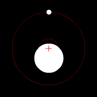
The spacecraft properties are a little more complex. For the ease of the calculations, its position will be based on the Earth. The injection define the position and speed applied to the spacecraft for it to transfer from a stable Low Earth Orbit to an orbit toward the Moon.

 1
 2
 3
 4
 5
 6
 7
 8
 9
10
11
12
13
14
15
16
17
18
19
20
21
22

## The Earth and the Moon properties are very similar

earth_pos = Vector(-barycenter_distance(EARTH_MOON_DISTANCE, EARTH_MASS, MOON_MASS), 0)
moon_pos = Vector(+barycenter_distance(EARTH_MOON_DISTANCE, MOON_MASS, EARTH_MASS), 0)

earth_vel = Vector.from_polar_rad(earth_pos.magnitude()*MOON_ANGULAR_SPEED, -math.pi/2)
moon_vel = Vector.from_polar_rad(moon_pos.magnitude()*MOON_ANGULAR_SPEED, math.pi/2)

earth = Body(EARTH_MASS, earth_pos, earth_vel)
moon = Body(MOON_MASS, moon_pos, moon_vel)

## The spacecraft properties are relative to the Earth

spacecraft_pos = earth_pos + Vector.from_polar_rad(
    EARTH_RADIUS+injection_altitude,
    injection_angle,
)
spacecraft_vel = Vector.from_polar_rad(
    orbital_speed(EARTH_MASS, (spacecraft_pos-earth_pos).magnitude()) + injection_dv,
    injection_angle+math.pi/2,
)
spacecraft = Body(1, spacecraft_pos, spacecraft_vel)

The spacecraft’s mass is not used, therefore it is set to 1, for safety, to avoid any division by zero.

The spacecraft’s velocity direction and position are a little hard to understand with the numbers, but with the following diagram it will be easier.

Simulation’s main loop

The two previous code snippets have set up the simulation, now comes the first part of the core of the simulation.

This code snippet loops on the given simulation time step sim_dt. It works in two steps: first, the acceleration is computed, without updating any position or velocity. Then, the velocity and position of each body is updated at the same time.

The loop would be a good place to save an history of the position of each body, in order to draw the trajectory once the simulation is finished.

 1
 2
 3
 4
 5
 6
 7
 8
 9
10
11
12
13
14
15
16
17
18

SIM_DURATION = 10.0*86400  # 10 days

sim_dt = 1.0 / sim_step_per_sec
last_sim_time = 0

while last_sim_time < SIM_DURATION:
    # compute the acceleration, without moving anything
    earth.update_acc([moon])
    moon.update_acc([earth])
    spacecraft.update_acc([earth, moon])

    # update the speed and position of everything
    earth.update_state(sim_dt)
    moon.update_state(sim_dt)
    spacecraft.update_state(sim_dt)

    # increase the simulation time by one step
    last_sim_time += sim_dt

A note about the while keyword used instead of the perhaps more suitable for keyword. I used it because it felt more suited for this particular case. The simulation and the export of the positions might not be synchronized, and I changed the logic many times. This way of doing was easier to rework and experiment with than a more classical for.

Euler integrator

This is the final code snippet, where all the magic happens. Do not skip this section too quickly, it is surprisingly easy to understand. Even if all the magic is here, it will not look like nonsensical incantations that are used to summon daemons.

As recalled from the previous code snippets, two functions are needed:

• update_acc() to update the acceleration
• update_state() to update the velocity and position

The update_state() function is very straightforward: with a basic engineering background, the Euler integrator should look familiar. The update_acc() function has a little more lines, but is also simple: it computes the acceleration by adding the gravitation from each body, using the equation for universal gravitation.

 1
 2
 3
 4
 5
 6
 7
 8
 9
10
11
12
13
14
15
16
17
18
19
20
21
22
23
24
25

class Body(object):
    def __init__(self, mass, pos, vel):
        self.mass = mass
        self.pos = pos
        self.vel = vel
        self.acc = Vector(0, 0)

    def update_acc(self, others):
        acc = Vector(0, 0)

        for other in others:
            dpos = other.pos - self.pos

            # force = newton = m*kg/s**2 VS acc = m/s**2
            grav_force = G*self.mass*other.mass / dpos.magnitude()**2
            grav_acc = grav_force / self.mass
            angle = math.atan2(dpos.y, dpos.x)

            acc += Vector.from_polar_rad(grav_acc, angle)

        self.acc = acc

    def update_state(self, sim_dt):
        self.vel += self.acc*sim_dt
        self.pos += self.vel*sim_dt

Checking the coherence of units is very helpful. The equation for universal gravitation is expressed in Newton which is m*kg/s**2, but the acceleration is expressed in m/s**2. It is clearly needed to divide by kg at some point, which makes sense to compute an acceleration.

There is another approximation here: the Earth is not a true sphere and the gravity is not constant everywhere. Real mission design will use a more precise model of the gravity of the Earth.

Full code

To keep the code short I have omitted a few non essential things: the definition of the constants (Earth and Moon properties, as well as some simulation parameters), the full Vector class (which does what you would expect and nothing more) and the export of the state (to plot the trajectory, a rather boring piece of code). There is definitely no hidden magic.

The code is a little long to show here (around 250 lines), but it is available here.

Output

When running this script, it outputs the following result.

 1
 2
 3
 4
 5
 6
 7
 8
 9
10
11
12
13
14
15
16
17
18
19
20
21

$ time python free-return-go.py -123.7 3150 0.1
Args
    injection_angle_deg: -123.700
    injection_dv: 3150.000
    sim_step_per_sec: 0.100

Pos
    Earth:      Vector(-4668173.198209003, 0)
    Moon:       Vector(379733826.801791, 0)
    Spacecraft: Vector(-8309617.175550222, -5460114.903542357)
Vel
    Earth:      Vector(7.614323001129578e-16, -12.435133144398803)
    Moon:       Vector(6.193891890800361e-14, 1011.5393099647653)
    Spacecraft: Vector(9104.2706956151, -6071.793776926436)

poss size: 17280
spacecraft pos -37398968 -320058357

real    0m3.157s
user    0m3.144s
sys     0m0.012s

Ignoring the debug prints, it says that it took a little more than 3 seconds⁶ to compute the final position of the spacecraft, which is (-37 398 968 ; -320 058 357) meters.

The code is configured to simulate 10 days and output the state of the spacecraft every 50 seconds, which gives us 17280 points. these states are written to a file, which can then be used to plot the trajectory of the spacecraft. This allow to run a lengthy but precise simulation and plot it quickly without simulating it again and again.

 1
 2
 3
 4
 5
 6
 7
 8
 9
10
11

$ head out.txt
t earth_x earth_y moon_x moon_y spacecraft_x spacecraft_y
0 -4668173 -124 379733827 10115 -8218061 -5520063
50 -4668173 -124 379733826 10115 -7753812 -5806941
100 -4668173 -124 379733825 10115 -7278831 -6073616
150 -4668173 -124 379733824 10115 -6794918 -6319495
200 -4668173 -124 379733824 10115 -6303916 -6544284
250 -4668173 -124 379733823 10115 -5807655 -6747980
300 -4668173 -124 379733822 10115 -5307894 -6930845
350 -4668173 -124 379733822 10115 -4806276 -7093376
400 -4668173 -124 379733821 10115 -4304299 -7236259

Our example can be plotted with this export of the positions. The following two diagrams show the same simulation, one with the trajectory of the spacecraft in a fixed frame (with respect to the Earth), and the other in a rotating frame (in order to keep the Moon fixed).

The Moon looks surprisingly close, although it is still several days away …

Exploring the parameter space

Now that I have a simulation tool, I wanted to know which trajectories were viable or not for a journey to the Moon. Why not run a few thousands simulations and find out what is the best strategy for outer-space travel?

A spacecraft beginning its journey to the Moon can tune two parameters to adjust its trajectory:

• Trans-lunar injection angle: where on the orbit (the angle Moon-Earth-spacecraft)
• Trans-lunar injection speed (or delta-v): how much energy is imparted to the spacecraft (the speed added to the initial orbital speed)

Here is again the schematic of the position and velocity of the spacecraft to really understand these two parameters.

Impact of the injection parameters

These two parameters are very chaotics: a small change will change the final position by a (much) large(r) amount. With just a few m/s or degrees, or even a tenth, the final position of the spacecraft will change by several hundreds of km. In real life, several mid-course correction maneuvers will take care of adjusting the trajectory to ensure a safe return and landing.

Here are a few examples showing the impact of varying these two parameters.

A crazy precision is required: an error as small as 0.1 m/s or 0.1 ° (0.1 deg corresponds to 1.5 sec in Low Earth Orbit) is the difference between a correct landing and big troubles (toasted and crashed, or simply frozen after a close Earth flyby: neither offer even the slightest survival chances). The diagrams shows a 200 km Low Earth Orbit. Do not try to find it on the first one, it is too close to the surface to be visible.

In order to perform a flyby of the Moon and come back to the Earth, the injection delta-v must be between 3 050 and 3 125 m/s (corresponding to a velocity between 10 840 and 10 920 m/s with respect to the Earth, for trajectories passing between 2 000 and 20 000 km from the Moon⁷). Empirically, the injection angle should be between 120 and 130 degrees.

Finding out how not to miss the Earth on the inbound journey

With this short explanation of the injection parameters, we can now try to answer the initial question: what is the outcome when these parameters are varied on a larger spectrum? What are the limits, and at which values does the spacecraft crashes on the Moon, injects into an heliocentric orbit or crashes on the Earth?

I ran a huge number of simulations (a few thousands) with different parameters: for each injection delta-v and angle I saved the closest approach to the Moon and the Earth. At around one second per simulation, it took a few minutes to have a rough idea and less than an hour for detailed results.

The result is plotted in 3D below. The horizontal plane is for the two parameters, and the vertical axis is used for the distance to the Earth: red for crashes, green for skimming through the atmosphere, grey for a close flyby and finally black for very far.

The two plots show the closest approach to the Moon and to the Earth. Since we want to focus on the safe return of our astronauts, we will focus on the Earth closest approach. The closest approach to the Moon is far less interesting, and any trajectory that end in the Earth atmosphere will pass by the Moon at a great distance (~10 000 km). In real life, the Moon closest approach would be very critical, due to landing site precision and safety requirements.

The graph shows that the injection angle affects less the result than the injection delta-v. The critical parameter is the injection delta-v: the “safe” entry distance (in green) happens only in a verry narrow window around 3150 m/s. The distances at the edge of the 4 grey-black zones are the usual satellite altitudes: <5 000 km (Low Earth Orbit) for most observation satellites, 20 000 km (Medium Earth Orbit) for GPS and 36 000 km (Geosynchronous Equatorial Orbit) for telecom.

A final note on the “safe” entry distance aforementioned: the green section of the plot corresponds to an altitude between 0 and 100 km. This value was chosen as a trade-off between fair approximation and being able to see something. Compared to real life, this is way too large, but otherwise we would not see anything. A real spacecraft would probably re-enter with a projected closest approach between something like 30 and 50 km⁸. Actually engineers do not focus on the closest approach (whose fancy name is perigee, when talking about the Earth), but rather on an entry interface. The entry interface specifications include the altitude, but also the speed and the angle of attack. A typical Apollo Earth entry interface was -6.5 degrees at 120 km altitude, with an acceptable range from 5.2 to -7.7 degrees⁹.

Conclusion

In this article, I presented the trajectory used by the Apollo missions in 1969 and the following years. This free-return trajectory allowed the astronauts to reach the Moon without compromising their safety in case of a serious issue. Apollo 13 took advantage of this feature to return safely to the Earth, without using the CSM (command and service module) main engine after the explosion of their oxygen tank, by fear that it could worsen the situation due to malfunction or even explosion. I also explained which methods can be used to simulate this trajectory, and how I implemented the one which uses the restricted circular three body problem. I showed how very small deviations of the input parameters (injection angle and delta-v) can have a huge impact on the return closest approach to the Earth.

Source code and data

I am a firm believer of open source, therefore the main source code used for the simulation can be found here, as well as all the code used to generate the diagrams and graphs. Since the simulator is rather slow, I also included the raw data that I used in my plots, so you can quickly plot and play with the data. You are welcome to explore and improve my work and send me any result you may find worth sharing!

Additional material

When writing this article, I found a some interesting material that I tough were worth sharing. Here they are:

• “Fly me to the Moon” by Jack Crenshaw: an awesome explanation of free-return trajectories, well worth reading even after this article - Original link and Webarchive link
• “Trajectories in the Earth-Moon space with symmetrical free return properties” by Arthur J. Schwaniger: advanced analysis of free-return trajectories, with some nice graphs - Orignal link
• “Introduction to Lunar Free-Return Trajectories” by Max Fagin: if you like videos - Youtube link
• “A Simple Targeting Procedure For Lunar Trans-Earth Injection” by Shane Robinson and David Geller: hard maths and trajectory optimization - Direct link, Original link

Upcoming article: optimization and benchmark

I initially wrote the simulator in Python, but was quickly put out by the slowness of the language. For calculation heavy applications like this one, Python is not the best choice. Nonetheless, it has allowed me to iterate quickly and promptly achieve a working prototype. It was also very easy to create plots of the results. I started trying to optimize the algorithm, but with Python it was hopeless. Since I am currently learning Rust, I started rewriting the simulator with this language. At this point I already had a few different versions and started comparing their speed. I went down a rabbit hole, and I plan to share my findings in an upcoming article that will probably be titled Free-return trajectory around the Moon: optimization and benchmark.